In this section, the different Ichthyop processes are described. These processes are implemented in the classes within the action folder.
Parameters associated with these processes must be included in action blocks. They can be activated or deactivated by setting the enabled tag (cf. Section 2.1).
6.1 Growth
There is 2 different implementations of the growth module. They can be selected by setting the class_name parameter in the action.growth action configuration block.
6.1.1 Linear growth
To use the linear growth method described in Lett et al. (2008), choose the LinearGrowthAction.java class.
Length increment is provided as follows:
\[
\Delta L = C_1 + C_2 \times \dfrac{F}{F + K_S} \times max(T, T_{thres}) \times \Delta t
\]
where \(\Delta t\) is the time-step (in days), \(C_1\) and \(C_2\) are parameters (coeff1 and coeff2), \(T_{thres}\) is a temperature threshold (threshold_temp parameter), \(F\) is the food quantity and \(K_S\) is a half-saturation constant (half_saturation parameter). If the latter is not defined or equals 0, \(Q\) is assumed to be \(1\).
The name of the food and temperature variables are provided by the food_field and temperature_field parameters.
6.1.2 Sole growth
If the {samp}SoleGrowthAction.java class is selected, the growth model used in Tanner et al. (2017) is used. It relies on the growth equation from Fonds (1979) and given by:
\[
\Delta L = C_1 \times T^{C_2} \times \Delta t
\]
with \(L\) the length, \(T\) the temperature and \(\Delta t\) the time step in days, and \(C_1\) and \(C_2\) are parameters (c1 and c2 respectively).
The temperature field is provided by the temperature_field parameter.
6.2 Lethal temperature and salinity
In Ichthyop, there is the possibility to define a range of temperature and salinity beyond which the particle is killed.
6.2.1 Lethal temperature
The functionning og the lethal temperature module depends on whether the growth module is enabled or not.
Growth disabled
lethal temperature can either be provided in a CSV file (lethal_temp_file parameter), which provides the lower and upper temperature values that can be supported by the particle as a function of age (in hours). The file must have the following format:
Time(hour);Cold temperature (C);Warm temperature (C)0;14;2248;13;2296;12;22
In this case, three age classes will be considered: \([0, 48[\), \([48, 96[\) and \([96, \infty[\)
If the lethal_temp_file parameter is not defined, single values will be used independently of the age. These values are provided in the cold_lethal_salinity_egg and warm_lethal_salinity_egg parameters.
Note that the temperature_field parameter, providing the name of the temperature variable, must also be provided.
Growth enabled
If the growth module is enabled, two cold and warm lethal temperatures must be provided. One for eggs (cold_lethal_temperature_egg and hot_lethal_temperature_egg), one for larva (cold_lethal_temperature_larva and hot_lethal_temperature_larva).
The stage (egg or larva) is determined by the growth module, and the right temperature range is applied to the particle.
6.2.2 Lethal salinity
Lethal salinity can either be provided in a CSV file (lethal_salt_file parameter), which provides the lower and upper salinity values that can be supported by the particle as a function of age (in hours). The file must have the following format:
In this case, three age classes will be considered: \([0, 48[\), \([48, 96[\) and \([96, \infty[\)
If the lethal_salt_file parameter is not defined, single values will be used independently of the age. These values are provided in the fresh_lethal_salinity_egg and saline_lethal_salinity_egg parameters.
Note that the salinity_field_ parameter, providing the name of the salinity variable, must also be provided.
6.3 Buoyancy
The buoyancy module allow to vertically displace a particle, depending on it’s density and on the sea water density, following Parada et al. (2003).
The buoyancy-induced vertical velocity of the particle is given by:
\[
W_{buoy} = \dfrac{1}{24} \times g \times a \times b \times \dfrac{\rho_{water} - \rho_{part}}{\rho_{water}} \mu^{-1} \log\left(2 \dfrac{a}{b} + 0.5\right);
\]
with \(a\) and \(b\) the semi-major axis and semi-minor axis of an ellipse (mean_major_axis and mean_minor_axis parameters), \(\mu\) the molecular viscosity (molecular_viscosity parameter), \(\rho_{water}\) the water density, \(\rho_{part}\) the particle density and \(g\) the gravitational acceleration (\(cm.s^{-2}\)).
If the particle density varies with age, it can be provided in a CSV file (density_file parameter), formatted as follows:
If the density_file parameter is not found, a constant density will be assumed (particle_density parameter).
The buoyancy process is only applied for the early life stages. If the growth process is disabled, it is controlled by the age_max parameter (provided in days). If this parameter is not provided, the buoyancy process will always be applied.
If the growth process is enabled, the application of the buoyancy module will be automatically managed.
6.4 Daily vertical migration
The MigrationAction.java manages the daily migration of the particles. It is done by providing daytime and nighttime depths, and the timing of the sunset and sunrise.
If the daytime_depth_file parameter is defined, it provides the depth of the particle during daytime. It is formatted as follows:
Age(day);Depth(m)0.0;-203.0;-255.0;-308.0;-35
If this parameter is not found, a constant daytime depth, provided by the daytime_depth parameter, is assumed.
Same thing for the nighttime depths, which can be set by either the nighttime_depth_file or the nighttime_depth parameters.
The sunset and sunrise hours are set by the sunset and sunrise parameters, which must have a HH::mm format.
If the growth module is deactivated, the user must provide the minimum age (in days) at which the particle starts to migrate (age_min parameter). If the growth module is activated, it manages the activation or deactivation of the daily migration.
Warning
When the target depth is greater than the total depth, the particle does not move.
6.5 Ontogenetic vertical migration
The ontogenetic migration module controls the migration to different habitats as a function of age. Its implementation in Ichthyop follows the CMS one. It uses the CMS configuration file (cms_ovm_config_file parameter), which is formatted as follows:
The first line provides the number of time steps in the CMS file, the second line provides the number of vertical levels in the CMS file. The third line provides the depth values and the fourth lines provides the time step values.
The remaining lines provide the probability matrix \(P_{z, t}\).
Note
The sum of the probability matrix along the depth dimension should equal 100.
At each time step, the index of the CMS time step, \(k\), is determined by comparing the simulation and CMS times as follows:
\[
t_{CMS}(k) < t \leq t_{CMS}(k + 1)
\]
When the CMS time index changes, all the particles are randomly distributed on the vertical, following the probability distribution of the given CMS time. If the CMS time index remains unchanged, nothing is done.
6.6 Wind drift
The wind-drift is implemented in the WindDriftFileAction.java class. This class requires that 2D (time, latitude, longitude) wind fields are provided. This is done by providing a input_path and a file_filter parameter, which specify the location and names of the wind files.
The user also provides field_time, wind_u, wind_v, longitude, latitude parameters, which specify the names of the time, zonal wind, meridional wind, longitude and latitude variables in the NetCDF files.
The user also provides a depth_application parameter, which specifies the depth at which the wind will impact the trajectories (only valid for 3D simulations), a wind_factor (\(F\), multiplication factor), an angle (\(\theta\)) and a wind_convention parameter (\(\varepsilon\), +1 if convention is ocean-based, i.e. wind-to, -1 if convention is atmospheric based, i.e. wind-from).
The changes in particle longitude (\(\lambda\)) and latitude (\(\phi\)) is provided as follows:
\(R\) is the Earth Radius and equals 6367.74 km. In the code, \(\dfrac{R \pi}{180}\), which is the distance in m of a 1 degree cell, is approximated to 111138 m
6.7 Random swimming
Ichthyop allows particles to randomly swim. This is achieved by using the SwimmingAction.java. The velocity may vary with the age of the particle.
The user provides a CSV absolute velocity file (velocity_file parameter), which must me formatted as follows:
Age (days);Speed (m/s)
0;0.1
5;0.2
15;0.3
The user also provides a boolean parameter (constant_velocity) that specifies whether the velocity should remain as defined in the CSV file, or if the absolute velocity should be randomly selected as follows:
\[
\|U\| = \|U\|_{file} \times \kappa
\]
with \(\kappa\) a random value in the \([0, 2]\) interval and \(\|U\|_{file}\) the velocity defined in the CSV file.
At each time-step, the zonal and meridonal velocities are defined as follows:
\[
U = \kappa' \varepsilon \|U\|
\]
\[
V = \varepsilon' \sqrt{\|U\|^2 - U^2}
\]
with \(\kappa'\) a random value between 0 and 1, and \(\varepsilon\) and \(\varepsilon'\) random values either equal to 1 or -1.
6.8 Wave drift
Ichthyop can take into account the effects of waves on the particles trajectories, following the Stokes drift equations of Stokes (2009):
\[
U_{S} = w \times k \times a^2 \times \exp\left(2 \times k \times z\right)
\]
In Ichthyop, the user provides zonal and meridional wave stokes drift and the wave periods. The horizontal displacement of particles is computed as follows:
\[
\Delta X = F \times U_{cur} \times \Delta t \times \exp\left(2 \times k_{wave} \times z\right)
\]
\[
\Delta Y = F \times V_{cur} \times \Delta t \times \exp\left(2 \times k_{wave} \times z\right)
\]
with \(U_{wave}\) and \(V_{wave}\) the zonal and meridional stokes components, \(T_{wave}\) the wave period, \(U_{cur}\) and \(V_{cur}\) the zonal and meridional ocean current components, \(z\) the depth and \(F\) a multiplication factor provided by the user.
6.9 Coastal behaviour
6.9.1 Bouncing
In the bouncing mode, the particle will bounce on the coast. First, whether the bouncing occurs on a meridional or a zonal coastline is determined.
In case of a meridional coastline, as shown in Figure 6.1, the calculation of the new position is performed as follows.
Let’s assume that the particle is at the position \((x, y)\) and is moved at the postion \((x + \Delta x, y + \Delta y)\). We suppose that
\[
\Delta y = \Delta y_1 + \Delta y_2,
\tag{6.1}\]
where \(\Delta y_1\) is the meridional distance between the particle and the coastline, and \(\Delta y_2\) is the distance that the particle will spend on land.
In the bouncing mode, the position increment can be written as
\[
\Delta_{cor} y = \Delta y_1 - \Delta y_2
\tag{6.2}\]
By replacing \(\Delta y_2\) using Equation 6.1, we can write:
\[
\Delta_{cor} y = \Delta y_1 - (\Delta y - \Delta y_1)
\]
\[
\Delta_{cor} y = 2 \Delta y_1 - \Delta y
\]
Figure 6.1: Coastal behaviour in bouncing mode.
6.10 Orientation
Active swimming has been implemented in Ichthyop following the work of Romain Chaput. Three active swimming behaviours have been implemented: the rheotaxis orientation (i.e. against the current), the cardinal orientation (i.e toward a given direction) and the reef orientation, i.e. orientation toward points of interests.
These three implementations involve the computation of a swimming velocity and direction. The former is common to all three methods, but the directions depend on the method considered.
6.10.1 Swimming velocity
The orientation processes all share common features. They both depend on a swimming velocity and random directions. The methods described below differ on the way the random directions are drafted.
Swimming velocity is computed following Staaterman, Paris, and Helgers (2012):
where \(I_{0}(\kappa)\) is the modified Bessel function of the first kind of order 0, \(\mu\) is angle where the distribution is centerred and \(\kappa\) is the concentration parameter. The distribution is as follows:
import matplotlib.pyplot as pltimport numpy as npfrom scipy.special import i0x = np.linspace(-np.pi, np.pi, 200)def von_misses(kappa): mu =0 y = np.exp(kappa*np.cos(x-mu))/(2*np.pi*i0(kappa))return yplt.figure()for i in [0.5, 1, 2, 5, 10, 20]: plt.plot(x, von_misses(i), label=f'$\kappa = {i}$')plt.legend()plt.xlim(x.min(), x.max())plt.show()
For computation purposes, all the Von Mises drafts performed in Ichthyop are done by using \(mu = 0\). The angles are thus centerred around 0. Then, the \(mu\) value is added.
Note
\(\theta = 0\) is eastward, \(\theta = \frac{\pi}{2}\) is northward, etc.
6.10.3 Computation of displacement
Given a swimming velocity \(V\) and a direction \(\theta\), the larva displacement (in \(m\)) is computed as follows:
\[
\Delta X = V \times \cos(\theta) \times \Delta t
\]
\[
\Delta Y = V \times \sin(\theta) \times \Delta t
\]
with \(\Delta t\) the time step. Next, the corresponding change in longitude (\(\lambda\)) and latitude (\(\varphi\)) is computed as follows:
In cardinal orientation, the user provides a fixed heading \(\theta_{card}\) and a fixed \(\kappa\) parameter. Then, at each time step, a new angle is randomly drafted following a Von Misses distribution \(f(\theta, \theta_{card}, \kappa)\).
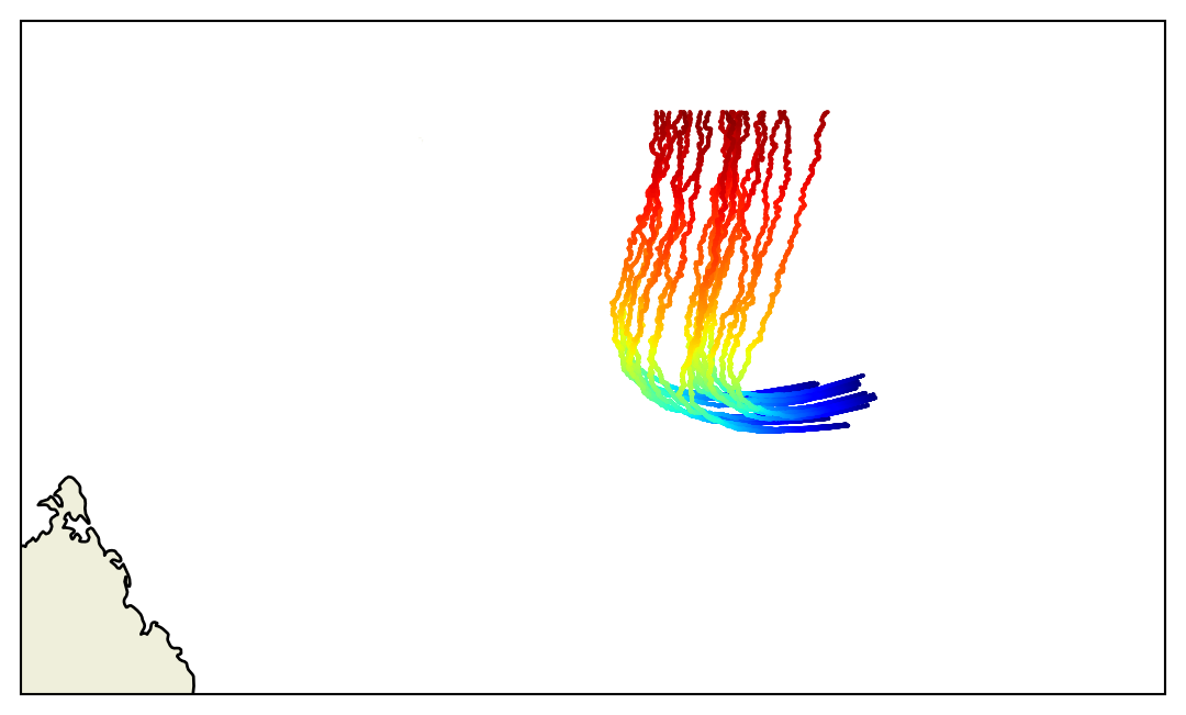
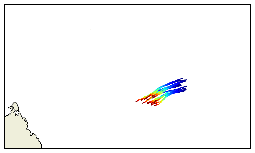
In the reef orientation method, the larva will target the closest target area (for instance coral reef). These areas are defined in an XML zone file by a polygon and a zone-specific \(\kappa\) parameter. The user also provides the sensory detection threshold of the larva (maximum detection distance \(\beta\)).
If the distance between the particle and the barycenter of the closest reef (\(D\)) is below the detection thereshold \(\beta\), the larva will swim in the direction of the reef.
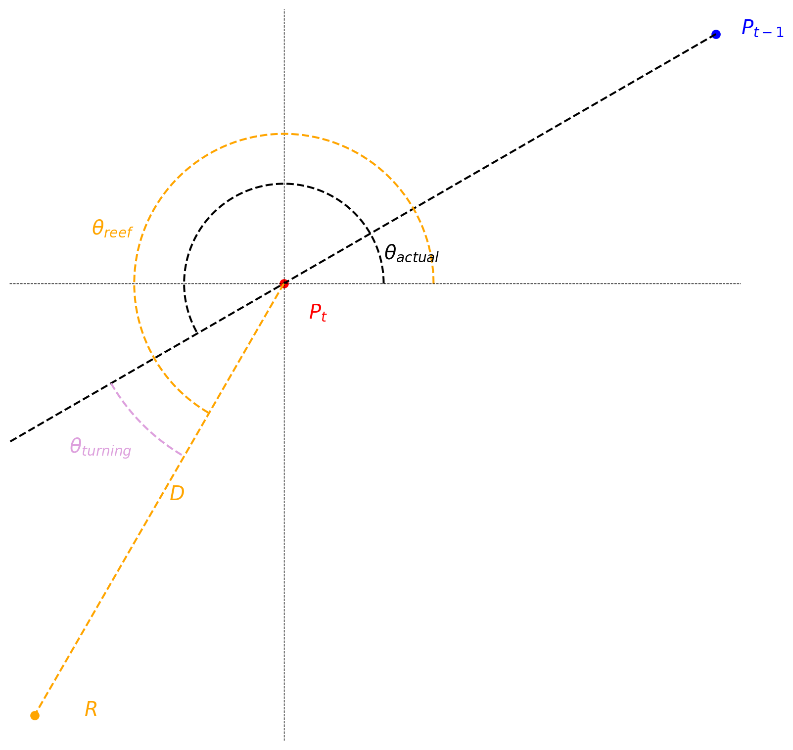
First, the angle of the current trajectory, \(\theta_{actual}\), is computed by using the particle position at the previous time step (blue point) and the actual position (red point).
\[
\Delta_X = (X_{t - 1} - X_{t})
\]
\[
\Delta_Y = (Y_{t - 1} - Y_{t})
\]
\[
\theta_{actual} = \arctan2(\Delta Y, \Delta X) + \pi
\]
The direction toward the reef, \(\theta_{reef}\) is also computed.
\[
\Delta_X = (X_{reef} - X_{t})
\]
\[
\Delta_Y = (Y_{reef} - Y_{t})
\]
\[
\theta_{reef} = \arctan2(\Delta Y, \Delta X)
\]
Warning
The angles are computed in the \((X, Y)\) space. Therefore, longitude and latitude coordinates are converted in \((X, Y)\) using the latlon2xy Dataset methods.
The turning angle \(\theta_{turning}\) is given by:
Therefore, the closest to the reef, the strongest the turning angle.
Then, a random angle is picked up following a Von Mises distribution \(f(\theta, \theta_{ponderated}, \kappa_{reef})\)
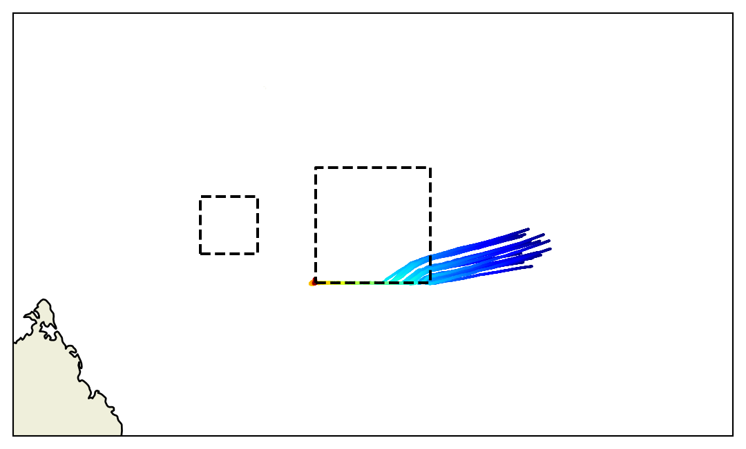
An example of a trajectory is provided below. In this case, two target destinations are provided (black boxes). The same \(\kappa\) value was used for both ares (1.2) and the \(\beta\) parameter has been set equal to 3 km.
Fonds, M. 1979. “Laboratory Observations on the Influence of Temperature and Salinity on Development of the Eggs and Growth of the Larvae of Solea Solea (Pisces).”Mar. Ecol. Prog. Ser 1 (9).
Lett, Christophe, Philippe Verley, Christian Mullon, Carolina Parada, Timothée Brochier, Pierrick Penven, and Bruno Blanke. 2008. “A Lagrangian Tool for Modelling Ichthyoplankton Dynamics.”Environmental Modelling & Software 23 (9): 1210–14. https://doi.org/https://doi.org/10.1016/j.envsoft.2008.02.005.
Parada, C, CD Van Der Lingen, C Mullon, and P Penven. 2003. “Modelling the Effect of Buoyancy on the Transport of Anchovy (Engraulis Capensis) Eggs from Spawning to Nursery Grounds in the Southern Benguela: An IBM Approach.”Fisheries Oceanography 12 (3): 170–84.
Staaterman, Erica, Claire B. Paris, and Judith Helgers. 2012. “Orientation Behavior in Fish Larvae: A Missing Piece to Hjort’s Critical Period Hypothesis.”Journal of Theoretical Biology 304 (July): 188–96. https://doi.org/10.1016/j.jtbi.2012.03.016.
Stokes, George Gabriel. 2009. “On the Theory of Oscillatory Waves.” In Mathematical and Physical Papers, 1:197–229. Cambridge Library Collection - Mathematics. Cambridge University Press. https://doi.org/10.1017/CBO9780511702242.013.
Tanner, Susanne E., Ana Teles-Machado, Filipe Martinho, Álvaro Peliz, and Henrique N. Cabral. 2017. “Modelling Larval Dispersal Dynamics of Common Sole (Solea Solea) Along the Western Iberian Coast.”Progress in Oceanography 156: 78–90. https://doi.org/https://doi.org/10.1016/j.pocean.2017.06.005.